


Highlights
- Stanislav is a Senior Quality Assurance Engineer at RingCentral.
- His team created its own performance testing tool.
- Stanislav shares insights on how the architecture of the tool was built and describes the entire process of the tool’s creation.
Introduction
Hi, my name is Stas (but you can call me Stan, if you like it better) and I am a Senior Quality Assurance Engineer at RingCentral Bulgaria. We develop an UCaaS solution for business communications. Specifically, my team is part of the Analytics department. The department’s main product is an analytics portal (all of a sudden, huh?) that can provide RingCentral customers with detailed information about calls, video meetings, webinars, rooms and devices. My team is responsible for telephony analytics: we develop and maintain some reports about call metrics and call quality within the analytics portal.
About two years ago our department in general and my team in particular started to develop a new call report. Normally, reports like ours are about some infrequent large queries to databases with their subsequent study and analysis. But in case of a new report, company protocols require us to perform some steps for production readiness validation. One of these steps is a performance test. So in the text below I will tell you our way of creating our own performance testing tool.
In this piece, I will describe my experience in general terms without much detail. I aim to show you exactly how to proceed and let you find your own way with my humble hints.
Infrastructure evolution
At the moment when our team realized that we definitely need a tool for performance testing, we’ve already had some work done. So here’s some background information on the relationship between us and performance tests.
An ace up my sleeve
As the Google Scholar project slogan says “Stand on the shoulders of giants”, I’m standing on the shoulders of my colleagues. As a performance testing tool, we’re using the Gatling plugin for sbt. The very first person to bring it to our project was my ex-teammate. Our team was migrating from one database to another, and we needed to somehow check the performance of a particular report, so we used the test results to make sure that the tested report worked well under pressure. But I should note that this wasn’t any kind of activity that would require the creation of an official report.
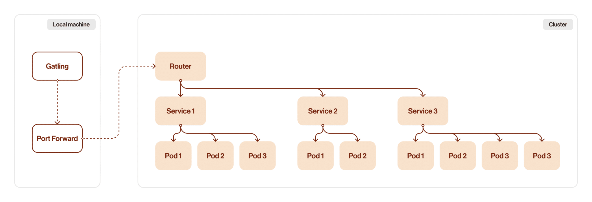
So what exactly did we have at that moment? It was a simple Scala class with a simple test for a specific method. This test used (and to be honest, the original code is still somewhere in the wilds of the repository, so I can say “uses”, by the way) the Kubernetes Port Forward method, which is often used to establish a connection between internal cluster resources and the local machine. I won’t explain how this method works, but I will say that this method has limitations that do not allow it to be used as a regular connection for performance testing purposes. As you can understand, I have replaced the Port Forward method with something else.
Revving up
As I mentioned above, I replaced the Port Forward method with another type of connection. I happened to have another project before this one. The main goal of that project was to create a set of tests to help our DevOps team verify an environment after a release deployment. Originally, port forwarding was used here as well, but our DevOps created an enhancement that allows some services to connect directly to cluster routers. So I used this new feature to increase the stability of these tests.
At the same time, this gave me an idea: what if I try to use this new connection type for a performance test? Theoretically, everything should be better: the throughput capacity should be higher than the port forward capacity. Stability should also be better. So I changed the connection scheme here. Let’s see the difference.
The image below shows the first version of the architecture.
The second image below shows the next version of the architecture.
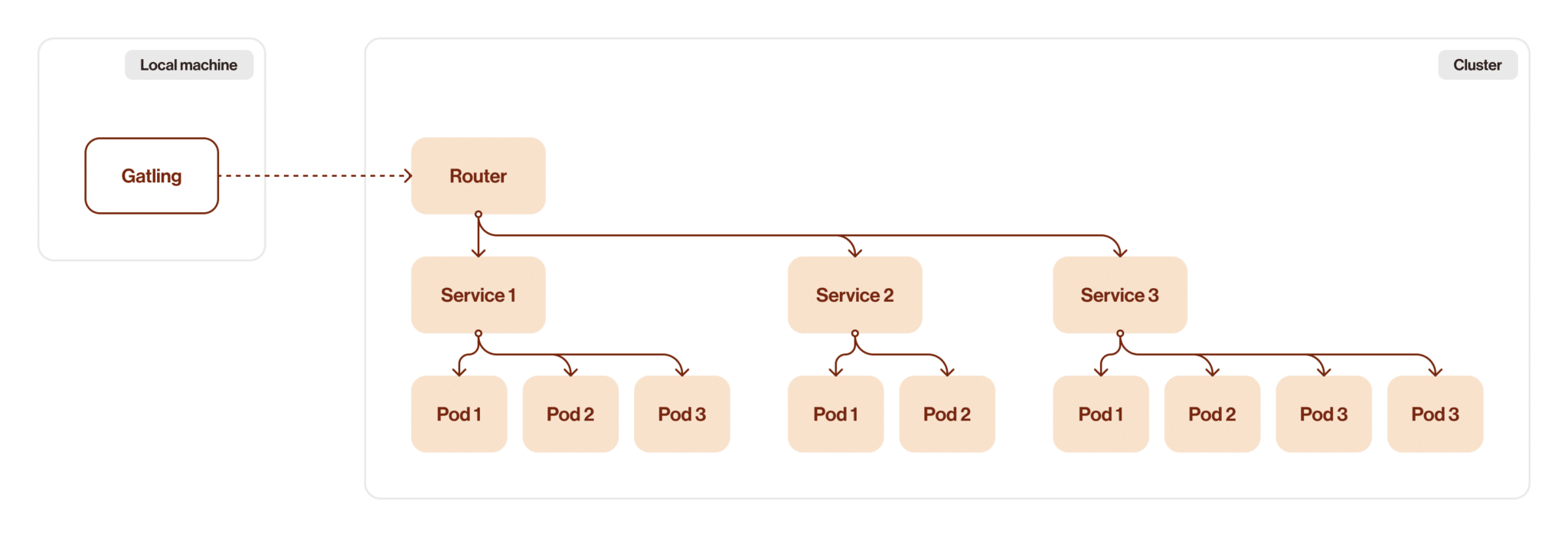
After this change I noticed that I got higher speed and channel capacity, but there are still network lags in this version, so I still have some room for improvement.
Above the klouds
As a next step I decided that it will be much better if our test module will be deployed to the cluster (klouds because clouds + kubernetes, don’t tell me you didn’t get it).
At this step we need to clarify the next thing: should it be a deployment or a job? Both ways have their own advantages. Deployment has advantages such as scalability (easy to scale up or down based on performance testing needs), resiliency (automatically replaces pods that fail, get deleted, or are terminated), and ease of update and rollback process. But if we take a look at the job benefits, the decision is easy: task completion focus (designed to run batch jobs to completion) and cleanup mechanism (job can delete produced work-in-progress artefacts).
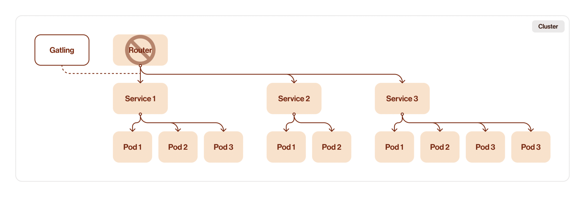
Let’s see what our architecture looks like after wrapping the test into the k8s job.
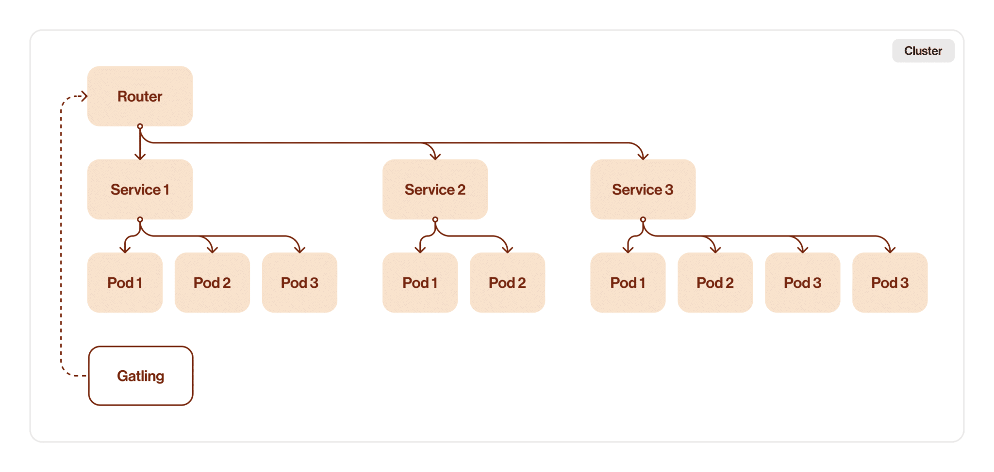
It looks good, I’d say it’s production ready, but it’s not. We still have a router as a bottleneck. And there’s a good chance that running an intensive performance test on a router will affect other members of the development team.
Kill the middleman
The final step in tuning the test architecture is to remove the last redundant part of our route between Gatling and a service. Since we have already deployed Gatling to the Kubernetes cluster, we just need to change some target configurations in the test source code and voila — we have excluded the router from our chain.
After all these changes, I think it’s time to look back and analyze our improvements.
Some boring numbers
If we want to understand what we’ve done after all, there’s no better way than to compare measurement results on each step. In the table below I will show you the difference, but before I should explain what exactly is placed in this table.
Gatling automatically divides responses in three groups by response time. There’re less than 800 ms (milliseconds), from 800 ms to 1200 ms and from 1200 ms and above. So the table will contain these three rows with percent of responses getting into this gap plus rows with failed responses count. And there’ll be three columns: measurements for the first architecture with port forward, for second iteration with router DNS and for the last one. I deliberately omit measurements of the penultimate stage because they’re not very revealing in my particular case. But it doesn’t mean that you can skip this step without any consequences.
| Port forward, % responses | Router DNS, % responses | Job in k8s, % responses | |
| t < 800 ms | 0% | 2% | 53% |
| 800 ms <= t < 1200 ms | 1% | 25% | 13% |
| t >= 1200 ms | 12% | 73% | 34% |
| failed | 87% | 0% | 0% |
As we can see, all our movements were not in vain. Buckle up, in the next part I’ll tell you more about the tests themselves and how we designed them.
Under the hood
We’ve talked about test infrastructure so far, but we haven’t said a word about what goes on inside our test container. You might be curious, so in the following part of my humble article, I will tell you more about performance testing itself.
Choose your fighter
One of the most important tasks for us was to understand which accounts to use for testing and how to select them. As I mentioned in the introduction, my team works with telephony data, so we measure all accounts in calls per day.
As you can see, the account ID is an important parameter for our test. Depending on it, we will get different amounts of calls in the same period of time, because obviously accounts have different rates of calls per day/week/month/year. At this point we realized that we need to divide all the accounts into some groups so that it’s possible to divide them into groups of similar size according to the amount of calls.
I think you can guess the purpose of this division, but I’ll explain it anyway. If an account has more calls in it, it will take up more space in a database, and responses with calls for this account will be heavier compared to smaller accounts. Given these facts, we should understand that if we mix large and small accounts, the averages will be skewed. So if we want to measure performance for a large account, we should use only large accounts to ensure the validity of the measurement data.
We have decided that three groups are sufficient for us: small, medium and large. In your case, the evaluation parameters and the number of groups may be different. But it doesn’t change the main idea — you should think carefully about whether the data should be divided in any way.
All in good time
Another important parameter for the test is time. Here we come to a few different problems. If we want to make some test runs in a single day, we should take into account that the call density isn’t uniform throughout the day. Also we should take into account that peak time is usually in a work day for our customers, most of which live in US/Canada time zones.
So if we don’t want to miss the right gap, we might do the next thing: adjust all to one timezone and declare in that zone the most interesting gaps. I think that the best timezone is UTC aka GMT+0. Adjusting all times to this specific one will help us avoid any time confusion.
But that’s not all problems with defining the time range. Performance testing is a tricky thing, you should consider many things and nuances. One of them is cache memory or just cache. Yep, the thing that usually helps you will now play against you. Let me explain where the devil hides.
Imagine that you want to test your service performance with processing monthly data. And the depth of data storage is one year. Here you will have 12 months of the data. But you don’t have to set a date range beginning only as the month beginning, right? Because if you set your gaps with whole months, you will get 12 gaps or even 11 because the day we are performing the test run might be in the middle of the month, so we wouldn’t count this part of the month. But here’s the moment when cache comes into play. You see, there’s only 12 (or 11) unique requests in terms of date range. That means, when your test will make a 13th request to the service, all possible responses will be processed at least one time. So response time will be corrupted with cache affection. Of course I don’t think that you will set ranges like these, it’s just an example.
But why is that bad? If you’re aiming to measure a single response time, there’s nothing bad. But in case if you have a lot more requests to run, you won’t get really much useful information. So how exactly do we trick the cache? The first option – disable it. Yes, that’s simple. But in case that you can’t, here’s the second option: use smaller units of time. I will show you how I’ve done it.
Let’s get back to our example. We have 12 months of data and are willing to measure response time for a monthly request. Maybe we should take day granularity? Then we’ll have 335 different gaps. I assume that the year has 365 days and the average month has 30 days, so we can take any day from today to the day that was 11 months ago as the end of the requested time range. And any day from a year ago to 1 month ago. Thus we obtain a moving month with a rather large spread. But if you’re going to make a lot more requests, you can downscale from days to hours. You will be able to get more than 7000 uniq time ranges.
Ugh, I was tired while I was writing this. Let’s talk about something easier for understanding (and explaining).
And what’s next?
The last step: define your simulation strategy. Sounds easy, huh? but that’s just at first glance. There’re a few types of simulation, but we’ll consider only three basic types of them here. They’re debug, border performance and stability. But before we talk about them let’s discuss some important terms.
I will use next terms in the following text:
- Intensity — number of requests per second to a service.
- Ramp duration — period of time when number of requests increases from current number of requests to another.
- Stage duration — period of time when number of requests is kept stable.
- Stage numbers — number of stage durations used in a particular test.
Now we’re ready to discuss different kinds of simulation. I will give some examples of values above for each type, but don’t mind changing them according to your needs.
Debug
The most simple and at the same time the most important type. It is used for debugging and testing the logic of the scripts themselves. I suggest using minimal static load in this case without any ramp. So the numbers will be Intensity = 1, Ramp duration = Null, Stage duration = 10 sec, Stage numbers = 1.
Border performance
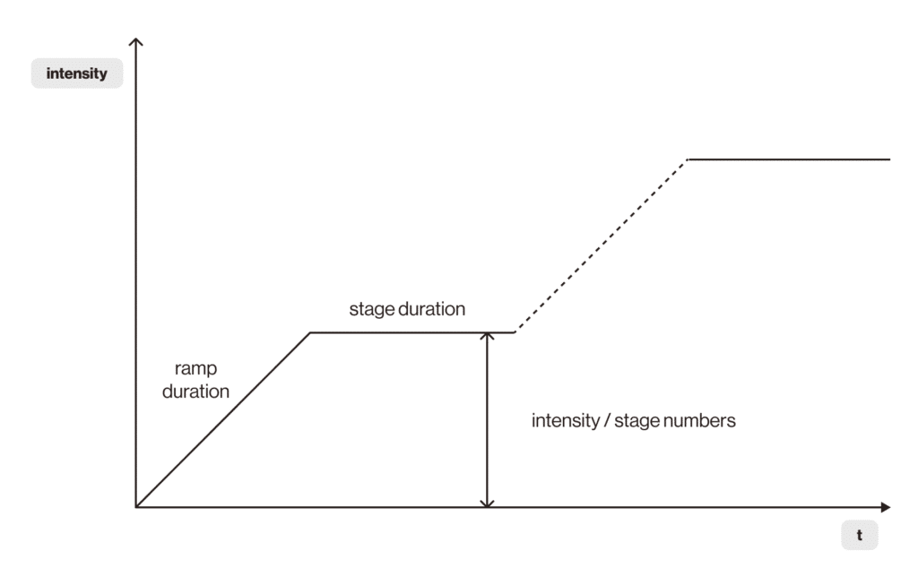
This simulation type is used to run tests with a step load. We use it to determine the points of maximum performance: increasing load with each step we can find an upper point of acceptable load for the service under test. Below is a graph that demonstrates how it works.
In the graph you can see the ramp duration of the load. The next load stage is reached during ramp duration. The stage itself lasts for stage duration, intensity per stage is calculated by the formula intensity / stage numbers. Here I won’t give you any exact numbers but I’ll give you some suggestions. First, adjust ramp duration. Increasing the load should be more gradual, so it will be easier to see where potential problems could be. But it should not be stretched too much either. Second, stage duration should not be shorter than ramp duration. You may adjust its length but I do not recommend to make it too short: deviations at the current load can be overlooked and this will blur the results for the next iteration.
Stability
This simulation type is used to run tests with a steadily supplied load with preliminary gradual overclocking. Such a test can be useful for confirming the stable operation of an application and performing regression tests. Below is an example of a steadily fed load test.
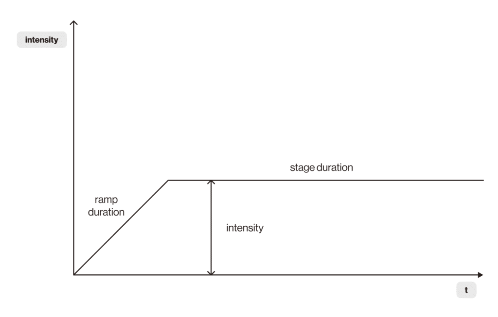
In the graph, you can see the stable load being supplied. Stable load is reached during ramp duration, stable load lasts during stage duration with fixed intensity. For better test utilization I suggest using some intelligence from production.
There were three main simulation types that were used in performance tests. Of course your limits end where your imagination ends, so never hesitate to experiment.
Aftertaste
Let’s summarize. I’ve talked about two big parts of the performance test: its infrastructure and its internal logic. Thanks for reading my whole stream of consciousness! I hope this material was useful and if you were thinking about starting performance testing on your project, you have a better understanding of what to do after this little reading.
Updated May 29, 2025